Exercise time: 45 minutes

Overview

Questions

How can I change the layout of a data frame?

Objectives

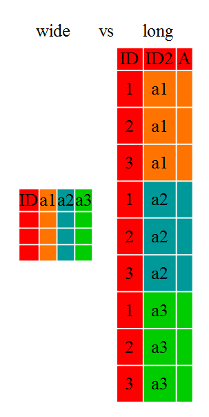
To understand the concepts of longer and wider data frame formats and be able to convert between them with tidyr.

Researchers often want to reshape their data frames from ‘wide’ to ‘longer’ layouts, or vice-versa. The ‘long’ layout or format is where:

each column is a variable
each row is an observation

In the purely ‘long’ (or ‘longest’) format, you usually have 1 column for the observed variable and the other columns are ID variables.

For the ‘wide’ format each row is often a site/subject/patient and you have multiple observation variables containing the same type of data. These can be either repeated observations over time, or observation of multiple variables (or a mix of both). You may find data input may be simpler or some other applications may prefer the ‘wide’ format.

However, many of R‘s functions have been designed assuming you have ’longer’ formatted data.

This tutorial will help you efficiently transform your data shape regardless of original format.

Long and wide data frame layouts mainly affect readability. For humans, the wide format is often more intuitive since we can often see more of the data on the screen due to its shape. However, the long format is more machine readable and is closer to the formatting of databases. The ID variables in our data frames are similar to the fields in a database and observed variables are like the database values.

Getting started

The `tidyr` package

Luckily, the tidyr package provides a number of very useful functions for reshaping data frames.

Tip: Tidyverse

tidyr package belongs to a broader family of opinionated R packages designed for data science called the “Tidyverse”. These packages are specifically designed to work harmoniously together. Some of these packages will be covered along this course, but you can find more complete information here: https://www.tidyverse.org/.

Or install the packages individually if you haven’t already done so (you may check with library("tidyr") & library("dplyr") )

Code

#install.packages("tidyr")
#install.packages("dplyr")   # in case you use pipe '%>%'

Load the packages

Code

library("tidyr")
library("dplyr")

Here we’re going to cover 5 of the most commonly used functions as well as using pipes (%>%) to combine them.

pivot_loger()
pivot_wider()
seperate()
unite()
NA removal

Load the gapminder data from the s link

Code

gapminder <- read.csv("https://raw.githubusercontent.com/swcarpentry/r-novice-gapminder/main/episodes/data/gapminder_data.csv")

First, lets look at the structure of our original gapminder data frame:

Code

head(gapminder)

country	year	pop	continent	lifeExp	gdpPercap
Afghanistan	1952	8425333	Asia	28.801	779.4453
Afghanistan	1957	9240934	Asia	30.332	820.8530
Afghanistan	1962	10267083	Asia	31.997	853.1007
Afghanistan	1967	11537966	Asia	34.020	836.1971
Afghanistan	1972	13079460	Asia	36.088	739.9811
Afghanistan	1977	14880372	Asia	38.438	786.1134

Code

# or str(gapminder)
# or View(gapminder)

Challenge 1

Is gapminder a purely long, purely wide, or some intermediate format?

Solution to challenge 1

The original gapminder data.frame is in an intermediate format. It is not
purely long since it had multiple observation variables
(`pop`,`lifeExp`,`gdpPercap`).

Sometimes, as with the gapminder dataset, we have multiple types of observed data. It is somewhere in between the purely ‘long’ and ‘wide’ data formats. We have 3 “ID variables” (continent, country, year) and 3 “Observation variables” (pop,lifeExp,gdpPercap). This intermediate format can be preferred despite not having ALL observations in 1 column given that all 3 observation variables have different units. There are few operations that would need us to make this data frame any longer (i.e. 4 ID variables and 1 Observation variable).

While using many of the functions in R, which are often vector based, you usually do not want to do mathematical operations on values with different units. For example, using the purely long format, a single mean for all of the values of population, life expectancy, and GDP would not be meaningful since it would return the mean of values with 3 incompatible units. The solution is that we first manipulate the data either by grouping (see the tomorrows lesson on dplyr), or we change the structure of the data frame.

Note:

Some plotting functions in R actually work better in the wide format data.

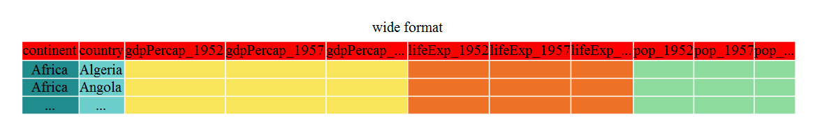
From wide to long format with `pivot_longer()`

Until now, we’ve been using the nicely formatted original gapminder dataset, but ‘real’ data (i.e. our own research data) will never be so well organized. Here let’s start with the wide formatted version of the gapminder dataset.

Tip

Download the wide version of the gapminder data from this link to a csv file and save it in your data folder.

We’ll load the data file and look at it. Note: we don’t want our continent and country columns to be factors, so we use the stringsAsFactors argument for read.csv() to disable that.

Code

gap_wide <- read.csv("https://raw.githubusercontent.com/swcarpentry/r-novice-gapminder/gh-pages/data/gapminder_wide.csv", stringsAsFactors = FALSE)

head(gap_wide)

continent	country	gdpPercap_1952	gdpPercap_1957	gdpPercap_1962	gdpPercap_1967	gdpPercap_1972	gdpPercap_1977	gdpPercap_1982	gdpPercap_1987	gdpPercap_1992	gdpPercap_1997	gdpPercap_2002	gdpPercap_2007	lifeExp_1952	lifeExp_1957	lifeExp_1962	lifeExp_1967	lifeExp_1972	lifeExp_1977	lifeExp_1982	lifeExp_1987	lifeExp_1992	lifeExp_1997	lifeExp_2002	lifeExp_2007	pop_1952	pop_1957	pop_1962	pop_1967	pop_1972	pop_1977	pop_1982	pop_1987	pop_1992	pop_1997	pop_2002	pop_2007
Africa	Algeria	2449.0082	3013.9760	2550.8169	3246.9918	4182.6638	4910.4168	5745.1602	5681.3585	5023.2166	4797.2951	5288.0404	6223.3675	43.077	45.685	48.303	51.407	54.518	58.014	61.368	65.799	67.744	69.152	70.994	72.301	9279525	10270856	11000948	12760499	14760787	17152804	20033753	23254956	26298373	29072015	31287142	33333216
Africa	Angola	3520.6103	3827.9405	4269.2767	5522.7764	5473.2880	3008.6474	2756.9537	2430.2083	2627.8457	2277.1409	2773.2873	4797.2313	30.015	31.999	34.000	35.985	37.928	39.483	39.942	39.906	40.647	40.963	41.003	42.731	4232095	4561361	4826015	5247469	5894858	6162675	7016384	7874230	8735988	9875024	10866106	12420476
Africa	Benin	1062.7522	959.6011	949.4991	1035.8314	1085.7969	1029.1613	1277.8976	1225.8560	1191.2077	1232.9753	1372.8779	1441.2849	38.223	40.358	42.618	44.885	47.014	49.190	50.904	52.337	53.919	54.777	54.406	56.728	1738315	1925173	2151895	2427334	2761407	3168267	3641603	4243788	4981671	6066080	7026113	8078314
Africa	Botswana	851.2411	918.2325	983.6540	1214.7093	2263.6111	3214.8578	4551.1421	6205.8839	7954.1116	8647.1423	11003.6051	12569.8518	47.622	49.618	51.520	53.298	56.024	59.319	61.484	63.622	62.745	52.556	46.634	50.728	442308	474639	512764	553541	619351	781472	970347	1151184	1342614	1536536	1630347	1639131
Africa	Burkina Faso	543.2552	617.1835	722.5120	794.8266	854.7360	743.3870	807.1986	912.0631	931.7528	946.2950	1037.6452	1217.0330	31.975	34.906	37.814	40.697	43.591	46.137	48.122	49.557	50.260	50.324	50.650	52.295	4469979	4713416	4919632	5127935	5433886	5889574	6634596	7586551	8878303	10352843	12251209	14326203
Africa	Burundi	339.2965	379.5646	355.2032	412.9775	464.0995	556.1033	559.6032	621.8188	631.6999	463.1151	446.4035	430.0707	39.031	40.533	42.045	43.548	44.057	45.910	47.471	48.211	44.736	45.326	47.360	49.580	2445618	2667518	2961915	3330989	3529983	3834415	4580410	5126023	5809236	6121610	7021078	8390505

Or try str(gap_wide)

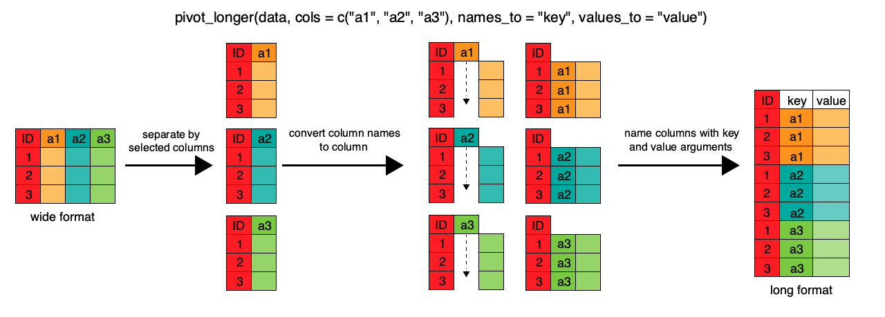
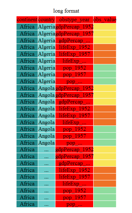
To change this very wide data frame layout back to our nice, intermediate (or longer) layout, we will use one of the two available pivot functions from the tidyr package. To convert from wide to a longer format, we will use the pivot_longer() function. pivot_longer() makes datasets longer by increasing the number of rows and decreasing the number of columns, or ‘lengthening’ your observation variables into a single variable.

Code

gap_long <- gap_wide %>%
  pivot_longer(
    cols = c(starts_with('pop'), starts_with('lifeExp'), starts_with('gdpPercap')),
    names_to = "obstype_year", values_to = "obs_values"
  )
head(gap_long)

continent	country	obstype_year	obs_values
Africa	Algeria	pop_1952	9279525
Africa	Algeria	pop_1957	10270856
Africa	Algeria	pop_1962	11000948
Africa	Algeria	pop_1967	12760499
Africa	Algeria	pop_1972	14760787
Africa	Algeria	pop_1977	17152804

Here we have used piping (%>%) syntax which is part of dplyr Package, we will see more tomorow at dplyr lesson too.

We first provide to pivot_longer() a vector of column names that will be pivoted into longer format. We could type out all the observation variables, but as in the select() function (see dplyr lesson if needed), we can use the starts_with() argument to select all variables that start with the desired character string. pivot_longer() also allows the alternative syntax of using the - symbol to identify which variables are not to be pivoted (i.e. ID variables).

The next arguments to pivot_longer() are names_to for naming the column that will contain the new ID variable (obstype_year) and values_to for naming the new amalgamated observation variable (obs_value). We supply these new column names as strings.

Apply the pivot_longer() and print the first few lines with head()

Code

gap_long <- gap_wide %>%
  pivot_longer(
    cols = c(-continent, -country),
    names_to = "obstype_year", values_to = "obs_values"
  )

head(gap_long)

continent	country	obstype_year	obs_values
Africa	Algeria	gdpPercap_1952	2449.008
Africa	Algeria	gdpPercap_1957	3013.976
Africa	Algeria	gdpPercap_1962	2550.817
Africa	Algeria	gdpPercap_1967	3246.992
Africa	Algeria	gdpPercap_1972	4182.664
Africa	Algeria	gdpPercap_1977	4910.417

Check the last couple of lines with tail()

Code

tail(gap_long)

continent	country	obstype_year	obs_values
Oceania	New Zealand	pop_1982	3210650
Oceania	New Zealand	pop_1987	3317166
Oceania	New Zealand	pop_1992	3437674
Oceania	New Zealand	pop_1997	3676187
Oceania	New Zealand	pop_2002	3908037
Oceania	New Zealand	pop_2007	4115771

That may seem trivial with this particular data frame, but sometimes you have 1 ID variable and 40 observation variables with irregular variable names. The flexibility is a huge time saver!

Split the variable into many with `seperate()`

Now obstype_year actually contains 2 pieces of information, the observation type (pop,lifeExp, or gdpPercap) and the year. We can use the separate() function to split the character strings into multiple variables

Code

gap_long <- gap_long %>% 
  separate(obstype_year, into = c('obs_type', 'year'), sep = "_")

gap_long$year <- as.integer(gap_long$year)

From long to intermediate format with `pivot_wider()`

It is always good to check work. So, let’s use the second pivot function, pivot_wider(), to ‘widen’ our observation variables back out. pivot_wider() is the opposite of pivot_longer(), making a dataset wider by increasing the number of columns and decreasing the number of rows. We can use pivot_wider() to pivot or reshape our gap_long to the original intermediate format or the widest format. Let’s start with the intermediate format.

The pivot_wider() function takes names_from and values_from arguments.

To names_from we supply the column name whose contents will be pivoted into new output columns in the widened data frame. The corresponding values will be added from the column named in the values_from argument.

Code

gap_normal <- gap_long %>%
  pivot_wider(names_from = obs_type, values_from = obs_values)
dim(gap_normal)

[1] 1704    6

Code

dim(gapminder)

[1] 1704    6

Code

names(gap_normal)

[1] "continent" "country"   "year"      "gdpPercap" "lifeExp"   "pop"

Code

names(gapminder)

[1] "country"   "year"      "pop"       "continent" "lifeExp"   "gdpPercap"

Now we’ve got an intermediate data frame gap_normal with the same dimensions as the original gapminder, but the order of the variables is different. Let’s fix that before checking if they are all.equal().

Code

gap_normal <- gap_normal[, names(gapminder)]
all.equal(gap_normal, gapminder)

[1] "Attributes: < Component \"class\": Lengths (3, 1) differ (string compare on first 1) >"
[2] "Attributes: < Component \"class\": 1 string mismatch >"                                
[3] "Component \"country\": 1704 string mismatches"                                         
[4] "Component \"pop\": Mean relative difference: 1.634504"                                 
[5] "Component \"continent\": 1212 string mismatches"                                       
[6] "Component \"lifeExp\": Mean relative difference: 0.203822"                             
[7] "Component \"gdpPercap\": Mean relative difference: 1.162302"

Code

head(gap_normal)

country	year	pop	continent	lifeExp	gdpPercap
Algeria	1952	9279525	Africa	43.077	2449.008
Algeria	1957	10270856	Africa	45.685	3013.976
Algeria	1962	11000948	Africa	48.303	2550.817
Algeria	1967	12760499	Africa	51.407	3246.992
Algeria	1972	14760787	Africa	54.518	4182.664
Algeria	1977	17152804	Africa	58.014	4910.417

Code

head(gapminder)

country	year	pop	continent	lifeExp	gdpPercap
Afghanistan	1952	8425333	Asia	28.801	779.4453
Afghanistan	1957	9240934	Asia	30.332	820.8530
Afghanistan	1962	10267083	Asia	31.997	853.1007
Afghanistan	1967	11537966	Asia	34.020	836.1971
Afghanistan	1972	13079460	Asia	36.088	739.9811
Afghanistan	1977	14880372	Asia	38.438	786.1134

We’re almost there, the original was sorted by country, then year.

Code

all.equal(gap_normal, gapminder)

[1] "Attributes: < Component \"class\": Lengths (3, 1) differ (string compare on first 1) >"
[2] "Attributes: < Component \"class\": 1 string mismatch >"                                
[3] "Component \"country\": 1704 string mismatches"                                         
[4] "Component \"pop\": Mean relative difference: 1.634504"                                 
[5] "Component \"continent\": 1212 string mismatches"                                       
[6] "Component \"lifeExp\": Mean relative difference: 0.203822"                             
[7] "Component \"gdpPercap\": Mean relative difference: 1.162302"

That’s great! We’ve gone from the longest format back to the intermediate and we didn’t introduce any errors in our code.

Join the variables into one with `unite()`

Now let’s convert the long all the way back to the wide. In the wide format, we will keep country and continent as ID variables and pivot the observations across the 3 metrics (pop,lifeExp,gdpPercap) and time (year). First we need to create appropriate labels for all our new variables (time*metric combinations) and we also need to unify our ID variables to simplify the process of defining gap_wide.

Code

gap_temp <- gap_long %>% unite(var_ID, continent, country, sep = "_")
str(gap_temp)

tibble [5,112 × 4] (S3: tbl_df/tbl/data.frame)
 $ var_ID    : chr [1:5112] "Africa_Algeria" "Africa_Algeria" "Africa_Algeria" "Africa_Algeria" ...
 $ obs_type  : chr [1:5112] "gdpPercap" "gdpPercap" "gdpPercap" "gdpPercap" ...
 $ year      : int [1:5112] 1952 1957 1962 1967 1972 1977 1982 1987 1992 1997 ...
 $ obs_values: num [1:5112] 2449 3014 2551 3247 4183 ...

Code

gap_temp <- gap_long %>%
    unite(ID_var, continent, country, sep = "_") %>%
    unite(var_names, obs_type, year, sep = "_")
str(gap_temp)

tibble [5,112 × 3] (S3: tbl_df/tbl/data.frame)
 $ ID_var    : chr [1:5112] "Africa_Algeria" "Africa_Algeria" "Africa_Algeria" "Africa_Algeria" ...
 $ var_names : chr [1:5112] "gdpPercap_1952" "gdpPercap_1957" "gdpPercap_1962" "gdpPercap_1967" ...
 $ obs_values: num [1:5112] 2449 3014 2551 3247 4183 ...

Using unite() we now have a single ID variable which is a combination of continent,country,and we have defined variable names. We’re now ready to pipe in pivot_wider()

Code

gap_wide_new <- gap_long %>%
  unite(ID_var, continent, country, sep = "_") %>%
  unite(var_names, obs_type, year, sep = "_") %>%
  pivot_wider(names_from = var_names, values_from = obs_values)
head(gap_wide_new)

ID_var	gdpPercap_1952	gdpPercap_1957	gdpPercap_1962	gdpPercap_1967	gdpPercap_1972	gdpPercap_1977	gdpPercap_1982	gdpPercap_1987	gdpPercap_1992	gdpPercap_1997	gdpPercap_2002	gdpPercap_2007	lifeExp_1952	lifeExp_1957	lifeExp_1962	lifeExp_1967	lifeExp_1972	lifeExp_1977	lifeExp_1982	lifeExp_1987	lifeExp_1992	lifeExp_1997	lifeExp_2002	lifeExp_2007	pop_1952	pop_1957	pop_1962	pop_1967	pop_1972	pop_1977	pop_1982	pop_1987	pop_1992	pop_1997	pop_2002	pop_2007
Africa_Algeria	2449.0082	3013.9760	2550.8169	3246.9918	4182.6638	4910.4168	5745.1602	5681.3585	5023.2166	4797.2951	5288.0404	6223.3675	43.077	45.685	48.303	51.407	54.518	58.014	61.368	65.799	67.744	69.152	70.994	72.301	9279525	10270856	11000948	12760499	14760787	17152804	20033753	23254956	26298373	29072015	31287142	33333216
Africa_Angola	3520.6103	3827.9405	4269.2767	5522.7764	5473.2880	3008.6474	2756.9537	2430.2083	2627.8457	2277.1409	2773.2873	4797.2313	30.015	31.999	34.000	35.985	37.928	39.483	39.942	39.906	40.647	40.963	41.003	42.731	4232095	4561361	4826015	5247469	5894858	6162675	7016384	7874230	8735988	9875024	10866106	12420476
Africa_Benin	1062.7522	959.6011	949.4991	1035.8314	1085.7969	1029.1613	1277.8976	1225.8560	1191.2077	1232.9753	1372.8779	1441.2849	38.223	40.358	42.618	44.885	47.014	49.190	50.904	52.337	53.919	54.777	54.406	56.728	1738315	1925173	2151895	2427334	2761407	3168267	3641603	4243788	4981671	6066080	7026113	8078314
Africa_Botswana	851.2411	918.2325	983.6540	1214.7093	2263.6111	3214.8578	4551.1421	6205.8839	7954.1116	8647.1423	11003.6051	12569.8518	47.622	49.618	51.520	53.298	56.024	59.319	61.484	63.622	62.745	52.556	46.634	50.728	442308	474639	512764	553541	619351	781472	970347	1151184	1342614	1536536	1630347	1639131
Africa_Burkina Faso	543.2552	617.1835	722.5120	794.8266	854.7360	743.3870	807.1986	912.0631	931.7528	946.2950	1037.6452	1217.0330	31.975	34.906	37.814	40.697	43.591	46.137	48.122	49.557	50.260	50.324	50.650	52.295	4469979	4713416	4919632	5127935	5433886	5889574	6634596	7586551	8878303	10352843	12251209	14326203
Africa_Burundi	339.2965	379.5646	355.2032	412.9775	464.0995	556.1033	559.6032	621.8188	631.6999	463.1151	446.4035	430.0707	39.031	40.533	42.045	43.548	44.057	45.910	47.471	48.211	44.736	45.326	47.360	49.580	2445618	2667518	2961915	3330989	3529983	3834415	4580410	5126023	5809236	6121610	7021078	8390505

Challenge 2

Take this 1 step further and create a gap_ludicrously_wide format data by pivoting over countries, year and the 3 metrics?

Hint

This new data frame should only have 5 rows.

Solution to challenge 2

Code

gap_ludicrously_wide <- gap_long %>%
   unite(var_names, obs_type, year, country, sep = "_") %>%
   pivot_wider(names_from = var_names, values_from = obs_values)

Now we have a great ‘wide’ format data frame, but the ID_var could be more usable, let’s separate it into 2 variables with separate()

Code

gap_wide_betterID <- separate(gap_wide_new, ID_var, c("continent", "country"), sep="_")
gap_wide_betterID <- gap_long %>%
    unite(ID_var, continent, country, sep = "_") %>%
    unite(var_names, obs_type, year, sep = "_") %>%
    pivot_wider(names_from = var_names, values_from = obs_values) %>%
    separate(ID_var, c("continent","country"), sep = "_")
str(gap_wide_betterID)

tibble [142 × 38] (S3: tbl_df/tbl/data.frame)
 $ continent     : chr [1:142] "Africa" "Africa" "Africa" "Africa" ...
 $ country       : chr [1:142] "Algeria" "Angola" "Benin" "Botswana" ...
 $ gdpPercap_1952: num [1:142] 2449 3521 1063 851 543 ...
 $ gdpPercap_1957: num [1:142] 3014 3828 960 918 617 ...
 $ gdpPercap_1962: num [1:142] 2551 4269 949 984 723 ...
 $ gdpPercap_1967: num [1:142] 3247 5523 1036 1215 795 ...
 $ gdpPercap_1972: num [1:142] 4183 5473 1086 2264 855 ...
 $ gdpPercap_1977: num [1:142] 4910 3009 1029 3215 743 ...
 $ gdpPercap_1982: num [1:142] 5745 2757 1278 4551 807 ...
 $ gdpPercap_1987: num [1:142] 5681 2430 1226 6206 912 ...
 $ gdpPercap_1992: num [1:142] 5023 2628 1191 7954 932 ...
 $ gdpPercap_1997: num [1:142] 4797 2277 1233 8647 946 ...
 $ gdpPercap_2002: num [1:142] 5288 2773 1373 11004 1038 ...
 $ gdpPercap_2007: num [1:142] 6223 4797 1441 12570 1217 ...
 $ lifeExp_1952  : num [1:142] 43.1 30 38.2 47.6 32 ...
 $ lifeExp_1957  : num [1:142] 45.7 32 40.4 49.6 34.9 ...
 $ lifeExp_1962  : num [1:142] 48.3 34 42.6 51.5 37.8 ...
 $ lifeExp_1967  : num [1:142] 51.4 36 44.9 53.3 40.7 ...
 $ lifeExp_1972  : num [1:142] 54.5 37.9 47 56 43.6 ...
 $ lifeExp_1977  : num [1:142] 58 39.5 49.2 59.3 46.1 ...
 $ lifeExp_1982  : num [1:142] 61.4 39.9 50.9 61.5 48.1 ...
 $ lifeExp_1987  : num [1:142] 65.8 39.9 52.3 63.6 49.6 ...
 $ lifeExp_1992  : num [1:142] 67.7 40.6 53.9 62.7 50.3 ...
 $ lifeExp_1997  : num [1:142] 69.2 41 54.8 52.6 50.3 ...
 $ lifeExp_2002  : num [1:142] 71 41 54.4 46.6 50.6 ...
 $ lifeExp_2007  : num [1:142] 72.3 42.7 56.7 50.7 52.3 ...
 $ pop_1952      : num [1:142] 9279525 4232095 1738315 442308 4469979 ...
 $ pop_1957      : num [1:142] 10270856 4561361 1925173 474639 4713416 ...
 $ pop_1962      : num [1:142] 11000948 4826015 2151895 512764 4919632 ...
 $ pop_1967      : num [1:142] 12760499 5247469 2427334 553541 5127935 ...
 $ pop_1972      : num [1:142] 14760787 5894858 2761407 619351 5433886 ...
 $ pop_1977      : num [1:142] 17152804 6162675 3168267 781472 5889574 ...
 $ pop_1982      : num [1:142] 20033753 7016384 3641603 970347 6634596 ...
 $ pop_1987      : num [1:142] 23254956 7874230 4243788 1151184 7586551 ...
 $ pop_1992      : num [1:142] 26298373 8735988 4981671 1342614 8878303 ...
 $ pop_1997      : num [1:142] 29072015 9875024 6066080 1536536 10352843 ...
 $ pop_2002      : num [1:142] 31287142 10866106 7026113 1630347 12251209 ...
 $ pop_2007      : num [1:142] 33333216 12420476 8078314 1639131 14326203 ...

Code

all.equal(gap_wide, gap_wide_betterID)

[1] "Attributes: < Component \"class\": Lengths (1, 3) differ (string compare on first 1) >"
[2] "Attributes: < Component \"class\": 1 string mismatch >"

There and back again!

Other great resources

R for Data Science (online book)
Data Wrangling Cheat sheet (pdf file)
Introduction to tidyr (online documentation)
Data wrangling with R and RStudio (online video)

Keypoints

Use the tidyr package to change the layout of data frames.
Use pivot_longer() to go from wide to longer layout.
Use pivot_wider() to go from long to wider layout.

R Session info

sessionInfo()

END

Overview

Getting started

The tidyr package

Challenge 1

From wide to long format with pivot_longer()

Split the variable into many with seperate()

From long to intermediate format with pivot_wider()

Join the variables into one with unite()

Challenge 2

Other great resources

Keypoints

R Session info

The `tidyr` package

From wide to long format with `pivot_longer()`

Split the variable into many with `seperate()`

From long to intermediate format with `pivot_wider()`

Join the variables into one with `unite()`