Manipulation of data frames means many things to many researchers: we often select certain observations (rows) or variables (columns), we often group the data by a certain variable(s), or we even calculate summary statistics. We can do these operations using the normal base R operations:
Code
mean(gapminder$gdpPercap[gapminder$continent =="Africa"]) # calculate average for African continent
But this isn’t very nice because there is a fair bit of repetition. Repeating yourself will cost you time, both now and later, and potentially introduce some nasty bugs.
The dplyr package
Luckily, the dplyr package provides a number of very useful functions for manipulating data frames in a way that will reduce the above repetition, reduce the probability of making errors, and probably even save you some typing. As an added bonus, you might even find the dplyr grammar easier to read.
Tip: Tidyverse
dplyr package belongs to a broader family of opinionated R packages designed for data science called the “Tidyverse”. These packages are specifically designed to work harmoniously together. Some of these packages will be covered along this course, but you can find more complete information here: https://www.tidyverse.org/.
Here we’re going to cover 5 of the most commonly used functions as well as using pipes (%>%) to combine them.
select()
filter()
group_by()
summarize()
mutate()
If you have have not installed this package earlier, please do so:
Code
# install.packages('dplyr')
Now let’s load the package:
Code
library("dplyr")
Using select()
If, for example, we wanted to move forward with only a few of the variables in our data frame we could use the select() function. This will keep only the variables you select.
Code
year_country_gdp <-select(gapminder, year, country, gdpPercap) # keep onöy certain columns
If we want to remove one column only from the gapminder data, for example, removing the continent column.
If we open up year_country_gdp we’ll see that it only contains the year, country and gdpPercap. Above we used ‘normal’ grammar, but the strengths of dplyr lie in combining several functions using pipes. Since the pipes grammar is unlike anything we’ve seen in R before, let’s repeat what we’ve done above using pipes.
Code
year_country_gdp <- gapminder %>%# use pipeselect(year, country, gdpPercap) # select few columns
To help you understand why we wrote that in that way, let’s walk through it step by step. First we summon the gapminder data frame and pass it on, using the pipe symbol %>%, to the next step, which is the select() function. In this case we don’t specify which data object we use in the select() function since in gets that from the previous pipe. Fun Fact: There is a good chance you have encountered pipes before in the shell. In R, a pipe symbol is %>% while in the shell it is | but the concept is the same!
Tip: Renaming data frame columns in dplyr
In Chapter 4 we covered how you can rename columns with base R by assigning a value to the output of the names() function. Just like select, this is a bit cumbersome, but thankfully dplyr has a rename() function.
Within a pipeline, the syntax is rename(new_name = old_name). For example, we may want to rename the gdpPercap column name from our select() statement above.
Code
tidy_gdp <- year_country_gdp %>%rename(gdp_per_capita = gdpPercap) # rename a variable name or column namehead(tidy_gdp) # see first few lines
year
country
gdp_per_capita
1952
Afghanistan
779.4453
1957
Afghanistan
820.8530
1962
Afghanistan
853.1007
1967
Afghanistan
836.1971
1972
Afghanistan
739.9811
1977
Afghanistan
786.1134
Using filter()
If we now want to move forward with the above, but only with European countries, we can combine select and filter
Code
year_country_gdp_euro <- gapminder %>%filter(continent =="Europe") %>%# keep observation (rows) that have Europeselect(year, country, gdpPercap) # keep variables
If we now want to show life expectancy of European countries but only for a specific year (e.g., 2007), we can do as below.
Code
europe_lifeExp_2007 <- gapminder %>%filter(continent =="Europe", year ==2007) %>%# now take observation that have Europe & 2007select(country, lifeExp)
Challenge 1
Write a single command (which can span multiple lines and includes pipes) that will produce a data frame that has the African values for lifeExp, country and year, but not for other Continents. How many rows does your data frame have and why?
As with last time, first we pass the gapminder data frame to the filter() function, then we pass the filtered version of the gapminder data frame to the select() function. Note: The order of operations is very important in this case. If we used ‘select’ first, filter would not be able to find the variable continent since we would have removed it in the previous step.
Using group_by()
Now, we were supposed to be reducing the error prone repetitiveness of what can be done with base R, but up to now we haven’t done that since we would have to repeat the above for each continent. Instead of filter(), which will only pass observations that meet your criteria (in the above: continent=="Europe"), we can use group_by(), which will essentially use every unique criteria that you could have used in filter.
You will notice that the structure of the data frame where we used group_by() (grouped_df) is not the same as the original gapminder (data.frame). A grouped_df can be thought of as a list where each item in the listis a data.frame which contains only the rows that correspond to the a particular value continent (at least in the example above).
Using summarize()
The above was a bit on the uneventful side but group_by() is much more exciting in conjunction with summarize(). This will allow us to create new variable(s) by using functions that repeat for each of the continent-specific data frames. That is to say, using the group_by() function, we split our original data frame into multiple pieces, then we can run functions (e.g. mean() or sd()) within summarize().
Another way to do this is to use the dplyr function arrange(), which arranges the rows in a data frame according to the order of one or more variables from the data frame. It has similar syntax to other functions from the dplyr package. You can use desc() inside arrange() to sort in descending order.
`summarise()` has grouped output by 'continent'. You can override using the
`.groups` argument.
count() and n()
A very common operation is to count the number of observations for each group. The dplyr package comes with two related functions that help with this.
For instance, if we wanted to check the number of countries included in the dataset for the year 2002, we can use the count() function. It takes the name of one or more columns that contain the groups we are interested in, and we can optionally sort the results in descending order by adding sort=TRUE:
Code
gapminder %>%filter(year ==2002) %>%count(continent, sort =TRUE) # do counting
continent
n
Africa
52
Asia
33
Europe
30
Americas
25
Oceania
2
If we need to use the number of observations in calculations, the n() function is useful. It will return the total number of observations in the current group rather than counting the number of observations in each group within a specific column. For instance, if we wanted to get the standard error of the life expectency per continent:
Code
gapminder %>%group_by(continent) %>%summarize(se_le =sd(lifeExp)/sqrt(n())) # calculaate standard error
continent
se_le
Africa
0.3663016
Americas
0.5395389
Asia
0.5962151
Europe
0.2863536
Oceania
0.7747759
You can also chain together several summary operations; in this case calculating the minimum, maximum, mean and se of each continent’s per-country life-expectancy:
`summarise()` has grouped output by 'continent'. You can override using the
`.groups` argument.
Connect mutate with logical filtering: ifelse
When creating new variables, we can hook this with a logical condition. A simple combination of mutate() and ifelse() facilitates filtering right where it is needed: in the moment of creating something new. This easy-to-read statement is a fast and powerful way of discarding certain data (even though the overall dimension of the data frame will not change) or for updating values depending on this given condition.
Code
## keeping all data but "filtering" after a certain condition# calculate GDP only for people with a life expectation above 25gdp_pop_bycontinents_byyear_above25 <- gapminder %>%mutate(gdp_billion =ifelse(lifeExp >25, # life expectation above 25 gdpPercap * pop /10^9, NA)) %>%# GDP (in billions)group_by(continent, year) %>%summarize(mean_gdpPercap =mean(gdpPercap),sd_gdpPercap =sd(gdpPercap),mean_pop =mean(pop),sd_pop =sd(pop),mean_gdp_billion =mean(gdp_billion),sd_gdp_billion =sd(gdp_billion))
`summarise()` has grouped output by 'continent'. You can override using the
`.groups` argument.
Code
## updating only if certain condition is fullfilled# for life expectations above 40 years, the gpd to be expected in the future is scaledgdp_future_bycontinents_byyear_high_lifeExp <- gapminder %>%mutate(gdp_futureExpectation =ifelse(lifeExp >40, gdpPercap *1.5, gdpPercap)) %>%group_by(continent, year) %>%summarize(mean_gdpPercap =mean(gdpPercap),mean_gdpPercap_expected =mean(gdp_futureExpectation))
`summarise()` has grouped output by 'continent'. You can override using the
`.groups` argument.
Combining dplyr and ggplot2
First install and load ggplot2:
Code
install.packages('ggplot2')
Code
library("ggplot2")
Warning: package 'ggplot2' was built under R version 4.4.3
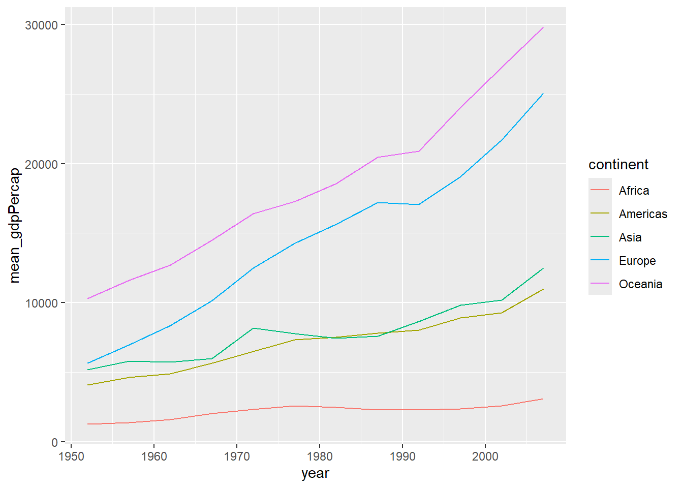
Let’s plot the variables from the last data you generated
Code
gdp_future_bycontinents_byyear_high_lifeExp %>%ggplot(mapping =aes(x = year, y = mean_gdpPercap, group = continent, colour = continent)) +geom_line()
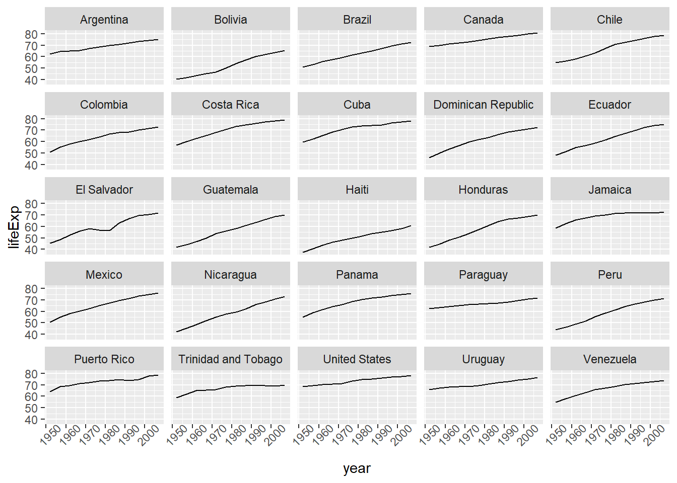
In the plotting lesson we looked at how to make a multi-panel figure by adding a layer of facet panels using ggplot2. Here is the code we used (with some extra comments):
Code
# Filter countries located in the Americasamericas <- gapminder[gapminder$continent =="Americas", ]# Make the plotggplot(data = americas, mapping =aes(x = year, y = lifeExp)) +geom_line() +facet_wrap( ~ country) +theme(axis.text.x =element_text(angle =45))
This code makes the right plot but it also creates an intermediate variable (americas) that we might not have any other uses for. Just as we used %>% to pipe data along a chain of dplyr functions we can use it to pass data to ggplot(). Because %>% replaces the first argument in a function we don’t need to specify the data = argument in the ggplot() function. By combining dplyr and ggplot2 functions we can make the same figure without creating any new variables or modifying the data.
Code
gapminder %>%# Filter countries located in the Americasfilter(continent =="Americas") %>%# Make the plotggplot(mapping =aes(x = year, y = lifeExp)) +# set x and ygeom_line() +# line plotfacet_wrap( ~ country) +# split the plot by countrytheme(axis.text.x =element_text(angle =45)) # x axis labels at 45 degree angle
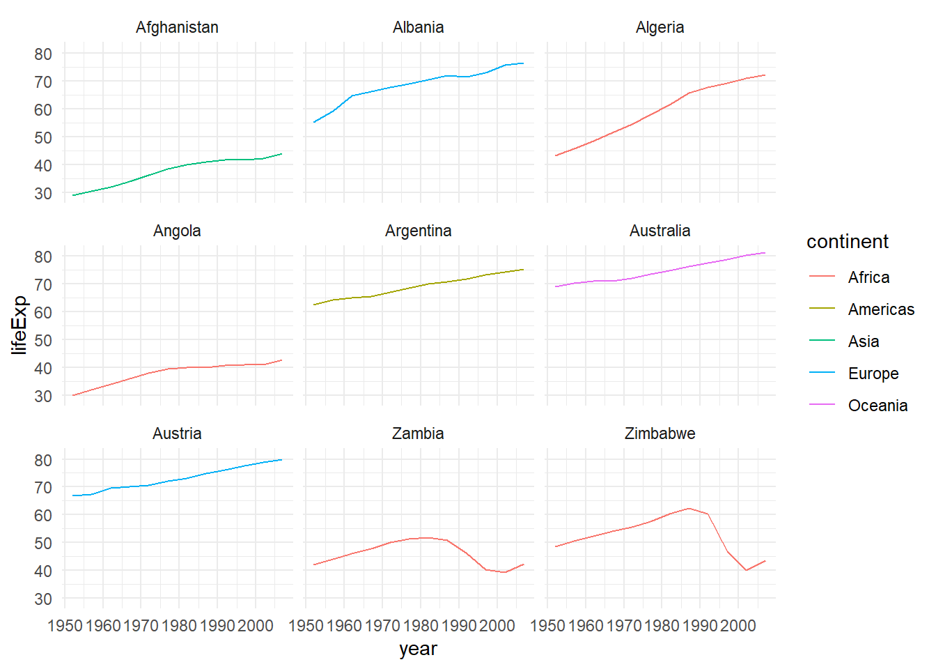
More examples of using the function mutate() and the ggplot2 package.
Code
gapminder %>%# extract first letter of country name into new columnmutate(startsWith =substr(country, 1, 1)) %>%# only keep countries starting with A or Zfilter(startsWith %in%c("A", "Z")) %>%# plot lifeExp into facetsggplot(aes(x = year, y = lifeExp, colour = continent)) +# x and y and set colorgeom_line() +# line plotfacet_wrap(vars(country)) +# faceting variables theme_minimal() # set theme
Advanced Challenge
Calculate the average life expectancy in 2002 of 2 randomly selected countries for each continent. Then arrange the continent names in reverse order. Hint: Use the dplyr functions arrange() and sample_n(), they have similar syntax to other dplyr functions.
Solution to Advanced Challenge
Code
lifeExp_2countries_bycontinents <- gapminder %>%# take the data filter(year==2002) %>%# keep rows that has year 2002group_by(continent) %>%# regroup by continentsample_n(2) %>%# take 2 random continentsummarize(mean_lifeExp=mean(lifeExp)) %>%# calculate mean life expectancyarrange(desc(mean_lifeExp)) # sort in reverse order
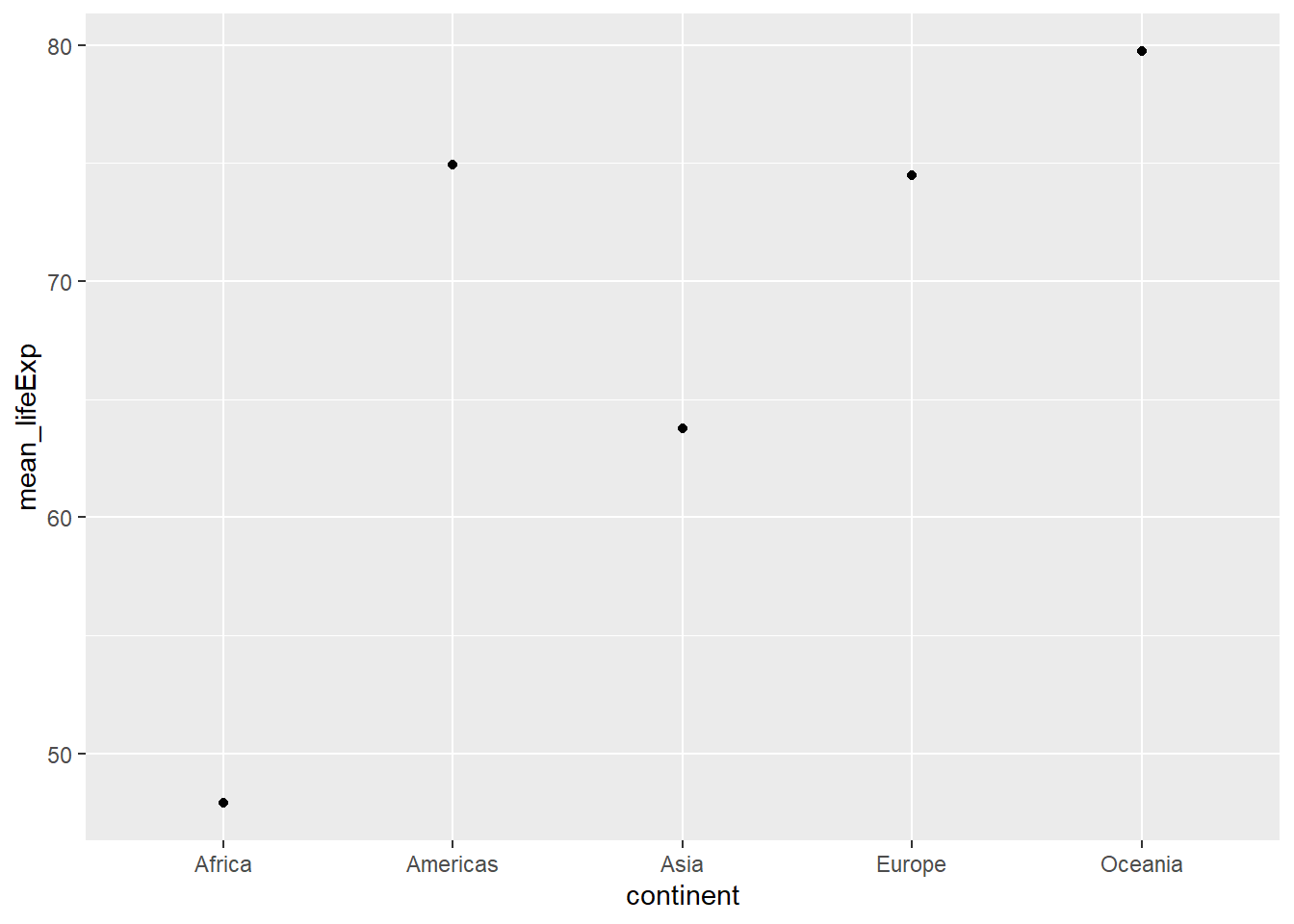
extras
Code
lifeExp_2countries_bycontinents %>%# dataggplot(aes(continent,mean_lifeExp)) +# x and y axisgeom_point() # scattered plot
Use select() to choose variables from a data frame.
Use filter() to choose data based on values.
Use group_by() and summarize() to work with subsets of data.
Use mutate() to create new variables.
R Session info
Code
sessionInfo()
R version 4.4.1 (2024-06-14 ucrt)
Platform: x86_64-w64-mingw32/x64
Running under: Windows 11 x64 (build 26100)

Matrix products: default


locale:
[1] LC_COLLATE=English_Sweden.utf8  LC_CTYPE=English_Sweden.utf8
[3] LC_MONETARY=English_Sweden.utf8 LC_NUMERIC=C
[5] LC_TIME=English_Sweden.utf8

time zone: Europe/Stockholm
tzcode source: internal

attached base packages:
[1] stats     graphics  grDevices utils     datasets  methods   base

other attached packages:
[1] ggplot2_4.0.0   dplyr_1.1.4     gapminder_1.0.1

loaded via a namespace (and not attached):
 [1] vctrs_0.6.5        cli_3.6.3          knitr_1.50         rlang_1.1.4
 [5] xfun_0.53          generics_0.1.4     S7_0.2.0           jsonlite_1.8.9
 [9] labeling_0.4.3     glue_1.8.0         htmltools_0.5.8.1  scales_1.4.0
[13] rmarkdown_2.29     grid_4.4.1         evaluate_1.0.5     tibble_3.2.1
[17] fastmap_1.2.0      yaml_2.3.10        lifecycle_1.0.4    compiler_4.4.1
[21] RColorBrewer_1.1-3 htmlwidgets_1.6.4  pkgconfig_2.0.3    rstudioapi_0.17.1
[25] farver_2.1.2       digest_0.6.37      R6_2.6.1           dichromat_2.0-0.1
[29] tidyselect_1.2.1   pillar_1.11.1      magrittr_2.0.3     gtable_0.3.6
[33] tools_4.4.1        withr_3.0.2
END
Source Code
---title: "Data Frame Manipulation with dplyr"editor: sourceformat: html: title-block-banner: true smooth-scroll: true toc: true toc-depth: 4 toc-location: right number-types: true number-depth: 4 code-fold: true code-tools: true code-copy: true code-overflow: wrap df-print: kable standalone: false fig-align: left theme: pulse highlight: kate---Exercise time: 55 minutes```{r}#| echo: false#| output: asiscat("# ","Overview")```**Questions**- How can I manipulate data frames without repeating myself?**Objectives**- To be able to use the six main data frame manipulation 'verbs' with pipes in `dplyr`.- To understand how `group_by()` and `summarize()` can be combined to summarize datasets.- Be able to analyze a subset of data using logical filtering.---------------------------------------------------------------```{r}# install.packages("gapminder") # install the package library(gapminder) # load the data# or import from your laptop# gapminder <- read.csv("data/gapminder_data.csv", header = TRUE)``````{r}str(gapminder) # see the data structure```Manipulation of data frames means many things to many researchers: we oftenselect certain observations (rows) or variables (columns), we often group thedata by a certain variable(s), or we even calculate summary statistics. We cando these operations using the normal base R operations:```{r}mean(gapminder$gdpPercap[gapminder$continent =="Africa"]) # calculate average for African continentmean(gapminder$gdpPercap[gapminder$continent =="Americas"])mean(gapminder$gdpPercap[gapminder$continent =="Asia"])```But this isn't very *nice* because there is a fair bit of repetition. Repeatingyourself will cost you time, both now and later, and potentially introduce somenasty bugs.## The `dplyr` packageLuckily, the [`dplyr`](https://cran.r-project.org/package=dplyr)package provides a number of very useful functions for manipulating data framesin a way that will reduce the above repetition, reduce the probability of makingerrors, and probably even save you some typing. As an added bonus, you mighteven find the `dplyr` grammar easier to read.::: {.callout-note}#### Tip: Tidyverse`dplyr` package belongs to a broader family of opinionated R packagesdesigned for data science called the "Tidyverse". Thesepackages are specifically designed to work harmoniously together.Some of these packages will be covered along this course, but you can find morecomplete information here: [https://www.tidyverse.org/](https://www.tidyverse.org/).:::Here we're going to cover 5 of the most commonly used functions as well as usingpipes (`%>%`) to combine them.1. `select()`2. `filter()`3. `group_by()`4. `summarize()`5. `mutate()`If you have have not installed this package earlier, please do so:```{r, eval=FALSE}# install.packages('dplyr')```Now let's load the package:```{r, message=FALSE}library("dplyr")```## Using select()If, for example, we wanted to move forward with only a few of the variables inour data frame we could use the `select()` function. This will keep only thevariables you select.```{r}year_country_gdp <-select(gapminder, year, country, gdpPercap) # keep onöy certain columns```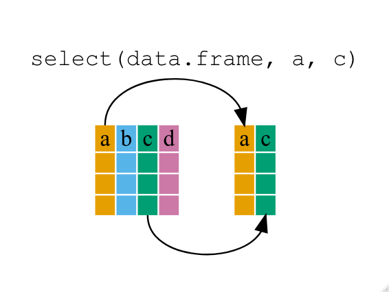{alt='Diagram illustrating use of select function to select two columns of a data frame'}If we want to remove one column only from the `gapminder` data, for example,removing the `continent` column.```{r}smaller_gapminder_data <-select(gapminder, -continent) # remove continent variable```If we open up `year_country_gdp` we'll see that it only contains the year,country and gdpPercap. Above we used 'normal' grammar, but the strengths of`dplyr` lie in combining several functions using pipes. Since the pipes grammaris unlike anything we've seen in R before, let's repeat what we've done aboveusing pipes.```{r}year_country_gdp <- gapminder %>%# use pipeselect(year, country, gdpPercap) # select few columns```To help you understand why we wrote that in that way, let's walk through it stepby step. First we summon the gapminder data frame and pass it on, using the pipesymbol `%>%`, to the next step, which is the `select()` function. In this casewe don't specify which data object we use in the `select()` function since ingets that from the previous pipe. **Fun Fact**: There is a good chance you haveencountered pipes before in the shell. In R, a pipe symbol is `%>%` while in theshell it is `|` but the concept is the same!::: {.callout-note}#### Tip: Renaming data frame columns in dplyrIn Chapter 4 we covered how you can rename columns with base R by assigning a value to the output of the `names()` function.Just like select, this is a bit cumbersome, but thankfully dplyr has a `rename()` function.Within a pipeline, the syntax is `rename(new_name = old_name)`.For example, we may want to rename the gdpPercap column name from our `select()` statement above.```{r}tidy_gdp <- year_country_gdp %>%rename(gdp_per_capita = gdpPercap) # rename a variable name or column namehead(tidy_gdp) # see first few lines```:::## Using filter()If we now want to move forward with the above, but only with Europeancountries, we can combine `select` and `filter````{r}year_country_gdp_euro <- gapminder %>%filter(continent =="Europe") %>%# keep observation (rows) that have Europeselect(year, country, gdpPercap) # keep variables```If we now want to show life expectancy of European countries but onlyfor a specific year (e.g., 2007), we can do as below.```{r}europe_lifeExp_2007 <- gapminder %>%filter(continent =="Europe", year ==2007) %>%# now take observation that have Europe & 2007select(country, lifeExp)```## Challenge 1Write a single command (which can span multiple lines and includes pipes) thatwill produce a data frame that has the African values for `lifeExp`, `country`and `year`, but not for other Continents. How many rows does your data framehave and why?::: {.callout-tip collapse="true"}#### Solution to challenge 1```{r}year_country_lifeExp_Africa <- gapminder %>%filter(continent =="Africa") %>%select(year, country, lifeExp)head(year_country_lifeExp_Africa)```:::As with last time, first we pass the gapminder data frame to the `filter()`function, then we pass the filtered version of the gapminder data frame to the`select()` function. **Note:** The order of operations is very important in thiscase. If we used 'select' first, filter would not be able to find the variablecontinent since we would have removed it in the previous step.## Using group_by()Now, we were supposed to be reducing the error prone repetitiveness of what canbe done with base R, but up to now we haven't done that since we would have torepeat the above for each continent. Instead of `filter()`, which will only passobservations that meet your criteria (in the above: `continent=="Europe"`), wecan use `group_by()`, which will essentially use every unique criteria that youcould have used in filter.```{r}str(gapminder)str(gapminder %>%group_by(continent))```You will notice that the structure of the data frame where we used `group_by()`(`grouped_df`) is not the same as the original `gapminder` (`data.frame`). A`grouped_df` can be thought of as a `list` where each item in the `list`is a`data.frame` which contains only the rows that correspond to the a particularvalue `continent` (at least in the example above).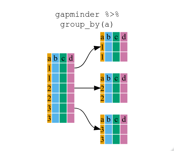{alt='Diagram illustrating how the group by function oraganizes a data frame into groups'}## Using summarize()The above was a bit on the uneventful side but `group_by()` is much moreexciting in conjunction with `summarize()`. This will allow us to create newvariable(s) by using functions that repeat for each of the continent-specificdata frames. That is to say, using the `group_by()` function, we split ouroriginal data frame into multiple pieces, then we can run functions(e.g. `mean()` or `sd()`) within `summarize()`.```{r}gdp_bycontinents <- gapminder %>%group_by(continent) %>%summarize(mean_gdpPercap =mean(gdpPercap))```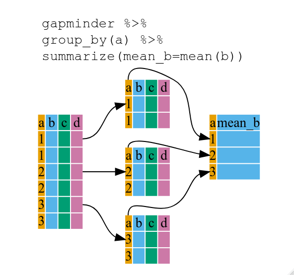{alt='Diagram illustrating the use of group by and summarize together to create a new variable'}```{r, eval=FALSE}continent mean_gdpPercap <fctr> <dbl>1 Africa 2193.7552 Americas 7136.1103 Asia 7902.1504 Europe 14469.4765 Oceania 18621.609```That allowed us to calculate the mean gdpPercap for each continent, but it getseven better.## Challenge 2Calculate the average life expectancy per country. Which has the longest average lifeexpectancy and which has the shortest average life expectancy?::: {.callout-tip collapse="true"}#### Solution to challenge 2```{r}lifeExp_bycountry <- gapminder %>%group_by(country) %>%# group countrywise contrywisesummarize(mean_lifeExp =mean(lifeExp)) # calculate averagelifeExp_bycountry %>%filter(mean_lifeExp ==min(mean_lifeExp) | mean_lifeExp ==max(mean_lifeExp))```Another way to do this is to use the `dplyr` function `arrange()`, whicharranges the rows in a data frame according to the order of one or morevariables from the data frame. It has similar syntax to other functions fromthe `dplyr` package. You can use `desc()` inside `arrange()` to sort indescending order.```{r}lifeExp_bycountry %>%arrange(mean_lifeExp) %>%# sorthead(1)lifeExp_bycountry %>%arrange(desc(mean_lifeExp)) %>%# arrange in decentralizing jonhead(1)```Alphabetical order works too```{r}lifeExp_bycountry %>%arrange(desc(country)) %>%head(1)```:::The function `group_by()` allows us to group by multiple variables. Let's group by `year` and `continent`.```{r}gdp_bycontinents_byyear <- gapminder %>%group_by(continent, year) %>%summarize(mean_gdpPercap =mean(gdpPercap))```That is already quite powerful, but it gets even better! You're not limited to defining 1 new variable in `summarize()`.```{r}gdp_pop_bycontinents_byyear <- gapminder %>%group_by(continent, year) %>%summarize(mean_gdpPercap =mean(gdpPercap),sd_gdpPercap =sd(gdpPercap), # calculate standard deviationmean_pop =mean(pop), # calculate averagesd_pop =sd(pop))```## count() and n()A very common operation is to count the number of observations for eachgroup. The `dplyr` package comes with two related functions that help with this.For instance, if we wanted to check the number of countries included in thedataset for the year 2002, we can use the `count()` function. It takes the nameof one or more columns that contain the groups we are interested in, and we canoptionally sort the results in descending order by adding `sort=TRUE`:```{r}gapminder %>%filter(year ==2002) %>%count(continent, sort =TRUE) # do counting```If we need to use the number of observations in calculations, the `n()` functionis useful. It will return the total number of observations in the current group rather than counting the number of observations in each group within a specific column. For instance, if we wanted to get the standard error of the life expectency per continent:```{r}gapminder %>%group_by(continent) %>%summarize(se_le =sd(lifeExp)/sqrt(n())) # calculaate standard error```You can also chain together several summary operations; in this case calculating the `minimum`, `maximum`, `mean` and `se` of each continent's per-country life-expectancy:```{r}gapminder %>%group_by(continent) %>%summarize(mean_le =mean(lifeExp),min_le =min(lifeExp),max_le =max(lifeExp),se_le =sd(lifeExp)/sqrt(n()))```## Using mutate()We can also create new variables prior to (or even after) summarizing information using `mutate()`.```{r}gdp_pop_bycontinents_byyear <- gapminder %>%mutate(gdp_billion = gdpPercap*pop/10^9) %>%group_by(continent,year) %>%summarize(mean_gdpPercap =mean(gdpPercap),sd_gdpPercap =sd(gdpPercap),mean_pop =mean(pop),sd_pop =sd(pop),mean_gdp_billion =mean(gdp_billion),sd_gdp_billion =sd(gdp_billion))```## Connect mutate with logical filtering: ifelseWhen creating new variables, we can hook this with a logical condition. A simple combination of`mutate()` and `ifelse()` facilitates filtering right where it is needed: in the moment of creating something new.This easy-to-read statement is a fast and powerful way of discarding certain data (even though the overall dimensionof the data frame will not change) or for updating values depending on this given condition.```{r}## keeping all data but "filtering" after a certain condition# calculate GDP only for people with a life expectation above 25gdp_pop_bycontinents_byyear_above25 <- gapminder %>%mutate(gdp_billion =ifelse(lifeExp >25, # life expectation above 25 gdpPercap * pop /10^9, NA)) %>%# GDP (in billions)group_by(continent, year) %>%summarize(mean_gdpPercap =mean(gdpPercap),sd_gdpPercap =sd(gdpPercap),mean_pop =mean(pop),sd_pop =sd(pop),mean_gdp_billion =mean(gdp_billion),sd_gdp_billion =sd(gdp_billion))## updating only if certain condition is fullfilled# for life expectations above 40 years, the gpd to be expected in the future is scaledgdp_future_bycontinents_byyear_high_lifeExp <- gapminder %>%mutate(gdp_futureExpectation =ifelse(lifeExp >40, gdpPercap *1.5, gdpPercap)) %>%group_by(continent, year) %>%summarize(mean_gdpPercap =mean(gdpPercap),mean_gdpPercap_expected =mean(gdp_futureExpectation))```## Combining `dplyr` and `ggplot2`First install and load ggplot2:```{r, eval=FALSE}install.packages('ggplot2')``````{r, message=FALSE}library("ggplot2")```Let's plot the variables from the last data you generated```{r}gdp_future_bycontinents_byyear_high_lifeExp %>%ggplot(mapping =aes(x = year, y = mean_gdpPercap, group = continent, colour = continent)) +geom_line() ```In the plotting lesson we looked at how to make a multi-panel figure by addinga layer of facet panels using `ggplot2`. Here is the code we used (with someextra comments):```{r}# Filter countries located in the Americasamericas <- gapminder[gapminder$continent =="Americas", ]# Make the plotggplot(data = americas, mapping =aes(x = year, y = lifeExp)) +geom_line() +facet_wrap( ~ country) +theme(axis.text.x =element_text(angle =45))```This code makes the right plot but it also creates an intermediate variable(`americas`) that we might not have any other uses for. Just as we used`%>%` to pipe data along a chain of `dplyr` functions we can use it to pass datato `ggplot()`. Because `%>%` replaces the first argument in a function we don'tneed to specify the `data =` argument in the `ggplot()` function. By combining`dplyr` and `ggplot2` functions we can make the same figure without creating anynew variables or modifying the data.```{r}gapminder %>%# Filter countries located in the Americasfilter(continent =="Americas") %>%# Make the plotggplot(mapping =aes(x = year, y = lifeExp)) +# set x and ygeom_line() +# line plotfacet_wrap( ~ country) +# split the plot by countrytheme(axis.text.x =element_text(angle =45)) # x axis labels at 45 degree angle```More examples of using the function `mutate()` and the `ggplot2` package.```{r}gapminder %>%# extract first letter of country name into new columnmutate(startsWith =substr(country, 1, 1)) %>%# only keep countries starting with A or Zfilter(startsWith %in%c("A", "Z")) %>%# plot lifeExp into facetsggplot(aes(x = year, y = lifeExp, colour = continent)) +# x and y and set colorgeom_line() +# line plotfacet_wrap(vars(country)) +# faceting variables theme_minimal() # set theme```## Advanced ChallengeCalculate the average life expectancy in 2002 of 2 randomly selected countriesfor each continent. Then arrange the continent names in reverse order.**Hint:** Use the `dplyr` functions `arrange()` and `sample_n()`, they havesimilar syntax to other dplyr functions.::: {.callout-tip collapse="true"}#### Solution to Advanced Challenge```{r}lifeExp_2countries_bycontinents <- gapminder %>%# take the data filter(year==2002) %>%# keep rows that has year 2002group_by(continent) %>%# regroup by continentsample_n(2) %>%# take 2 random continentsummarize(mean_lifeExp=mean(lifeExp)) %>%# calculate mean life expectancyarrange(desc(mean_lifeExp)) # sort in reverse order```:::### extras```{r}lifeExp_2countries_bycontinents %>%# dataggplot(aes(continent,mean_lifeExp)) +# x and y axisgeom_point() # scattered plot```## Other great resources- [R for Data Science](https://r4ds.hadley.nz/) (online book)- [Data Wrangling Cheat sheet](https://www.rstudio.com/wp-content/uploads/2015/02/data-wrangling-cheatsheet.pdf) (pdf file)- [Introduction to dplyr](https://dplyr.tidyverse.org/) (online documentation)- [Data wrangling with R and RStudio](https://www.rstudio.com/resources/webinars/data-wrangling-with-r-and-rstudio/) (online video)- [Tidyverse Skills for Data Science](https://jhudatascience.org/tidyversecourse/) (online book)## keypoints- Use the `dplyr` package to manipulate data frames.- Use `select()` to choose variables from a data frame.- Use `filter()` to choose data based on values.- Use `group_by()` and `summarize()` to work with subsets of data.- Use `mutate()` to create new variables.#### R Session info```{r}sessionInfo()```############## END